Data generation mechanism

This example illustrates the Geometric SMOTE data generation mechanism and the usage of its hyperparameters.

# Author: Georgios Douzas <gdouzas@icloud.com>
# Licence: MIT

import numpy as np
import matplotlib.pyplot as plt

from sklearn.datasets import make_blobs
from imblearn.over_sampling import SMOTE

from gsmote import GeometricSMOTE

print(__doc__)

XLIM, YLIM = [-3.0, 3.0], [0.0, 4.0]
RANDOM_STATE = 5


def generate_imbalanced_data(
    n_maj_samples, n_min_samples, centers, cluster_std, *min_point
):
    """Generate imbalanced data."""
    X_neg, _ = make_blobs(
        n_samples=n_maj_samples,
        centers=centers,
        cluster_std=cluster_std,
        random_state=RANDOM_STATE,
    )
    X_pos = np.array(min_point)
    X = np.vstack([X_neg, X_pos])
    y_pos = np.zeros(X_neg.shape[0], dtype=np.int8)
    y_neg = np.ones(n_min_samples, dtype=np.int8)
    y = np.hstack([y_pos, y_neg])
    return X, y


def plot_scatter(X, y, title):
    """Function to plot some data as a scatter plot."""
    plt.figure()
    plt.scatter(X[y == 1, 0], X[y == 1, 1], label='Positive Class')
    plt.scatter(X[y == 0, 0], X[y == 0, 1], label='Negative Class')
    plt.xlim(*XLIM)
    plt.ylim(*YLIM)
    plt.gca().set_aspect('equal', adjustable='box')
    plt.legend()
    plt.title(title)


def plot_hyperparameters(oversampler, X, y, param, vals, n_subplots):
    """Function to plot resampled data for various
    values of a geometric hyperparameter."""
    n_rows = n_subplots[0]
    fig, ax_arr = plt.subplots(*n_subplots, figsize=(15, 7 if n_rows > 1 else 3.5))
    if n_rows > 1:
        ax_arr = [ax for axs in ax_arr for ax in axs]
    for ax, val in zip(ax_arr, vals):
        oversampler.set_params(**{param: val})
        X_res, y_res = oversampler.fit_resample(X, y)
        ax.scatter(X_res[y_res == 1, 0], X_res[y_res == 1, 1], label='Positive Class')
        ax.scatter(X_res[y_res == 0, 0], X_res[y_res == 0, 1], label='Negative Class')
        ax.set_title(f'{val}')
        ax.set_xlim(*XLIM)
        ax.set_ylim(*YLIM)


def plot_comparison(oversamplers, X, y):
    """Function to compare SMOTE and Geometric SMOTE
    generation of noisy samples."""
    fig, ax_arr = plt.subplots(1, 2, figsize=(15, 5))
    for ax, (name, ovs) in zip(ax_arr, oversamplers):
        X_res, y_res = ovs.fit_resample(X, y)
        ax.scatter(X_res[y_res == 1, 0], X_res[y_res == 1, 1], label='Positive Class')
        ax.scatter(X_res[y_res == 0, 0], X_res[y_res == 0, 1], label='Negative Class')
        ax.set_title(name)
        ax.set_xlim(*XLIM)
        ax.set_ylim(*YLIM)

Generate imbalanced data

We are generating a highly imbalanced non Gaussian data set. Only two samples from the minority (positive) class are included to illustrate the Geometric SMOTE data generation mechanism.

X, y = generate_imbalanced_data(
    200, 2, [(-2.0, 2.25), (1.0, 2.0)], 0.25, [-0.7, 2.3], [-0.5, 3.1]
)
plot_scatter(X, y, 'Imbalanced data')

Geometric hyperparameters

Similarly to SMOTE and its variations, Geometric SMOTE uses the k_neighbors hyperparameter to select a random neighbor among the k nearest neighbors of a minority class instance. On the other hand, Geometric SMOTE expands the data generation area from the line segment of the SMOTE mechanism to a hypersphere that can be truncated and deformed. The characteristics of the above geometric area are determined by the hyperparameters truncation_factor, deformation_factor and selection_strategy. These are called geometric hyperparameters and allow the generation of diverse synthetic data as shown below.

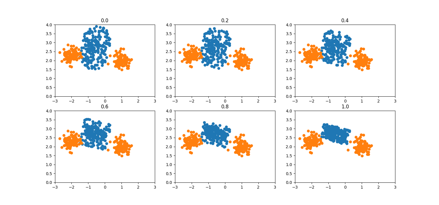
Truncation factor

The hyperparameter truncation_factor determines the degree of truncation that is applied on the initial geometric area. Selecting the values of geometric hyperparameters as truncation_factor=0.0, deformation_factor=0.0 and selection_strategy='minority', the data generation area in 2D corresponds to a circle with center as one of the two minority class samples and radius equal to the distance between them. In the multi-dimensional case the corresponding area is a hypersphere. 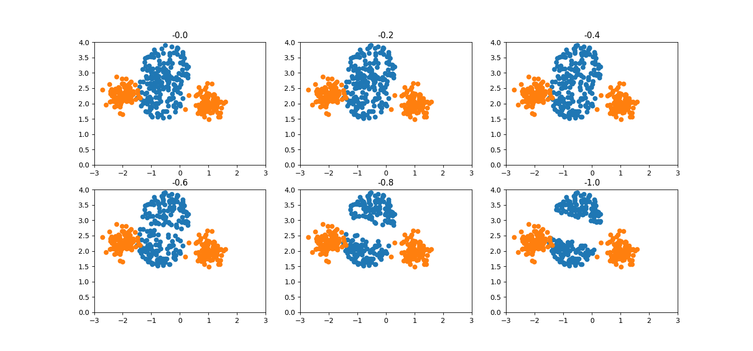When truncation factor is increased, the hypersphere is truncated and for truncation_factor=1.0 becomes a half-hypersphere. Negative values of truncation_factor have a similar effect but on the opposite direction.

gsmote = GeometricSMOTE(
    k_neighbors=1,
    deformation_factor=0.0,
    selection_strategy='minority',
    random_state=RANDOM_STATE,
)
truncation_factors = np.array([0.0, 0.2, 0.4, 0.6, 0.8, 1.0])
n_subplots = [2, 3]
plot_hyperparameters(gsmote, X, y, 'truncation_factor', truncation_factors, n_subplots)
plot_hyperparameters(gsmote, X, y, 'truncation_factor', -truncation_factors, n_subplots)

• 
• 

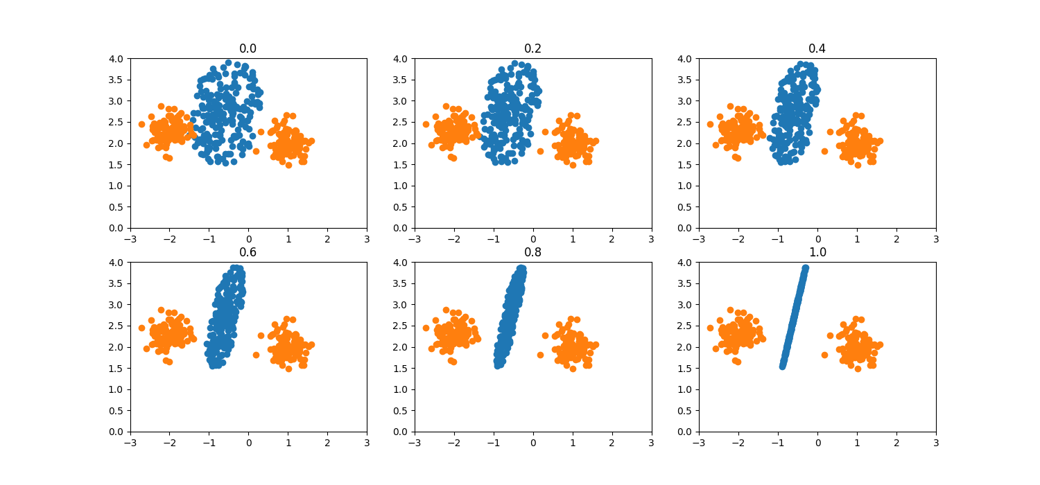
Deformation factor

When the deformation_factor is increased, the data generation area deforms to an ellipsis and for deformation_factor=1.0 becomes a line segment.

gsmote = GeometricSMOTE(
    k_neighbors=1,
    truncation_factor=0.0,
    selection_strategy='minority',
    random_state=RANDOM_STATE,
)
deformation_factors = np.array([0.0, 0.2, 0.4, 0.6, 0.8, 1.0])
n_subplots = [2, 3]
plot_hyperparameters(gsmote, X, y, 'deformation_factor', truncation_factors, n_subplots)

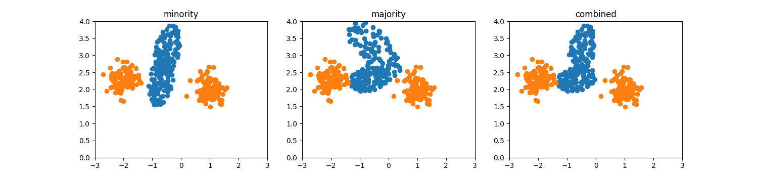
Selection strategy

The hyperparameter selection_strategy determines the selection mechanism of nearest neighbors. Initially, a minority class sample is selected randomly. When selection_strategy='minority', a second minority class sample is selected as one of the k nearest neighbors of it. For selection_strategy='majority', the second sample is its nearest majority class neighbor. Finally, for selection_strategy='combined' the two selection mechanisms are combined and the second sample is the nearest to the first between the two samples defined above.

gsmote = GeometricSMOTE(
    k_neighbors=1,
    truncation_factor=0.0,
    deformation_factor=0.5,
    random_state=RANDOM_STATE,
)
selection_strategies = np.array(['minority', 'majority', 'combined'])
n_subplots = [1, 3]
plot_hyperparameters(
    gsmote, X, y, 'selection_strategy', selection_strategies, n_subplots
)

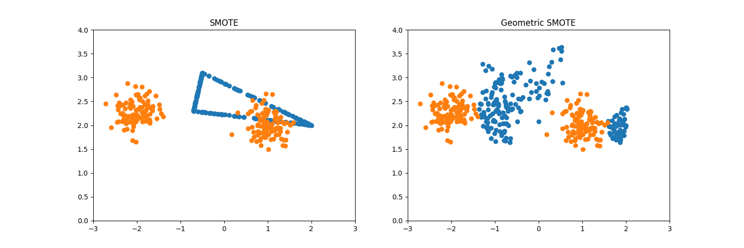
Noisy samples

We are adding a third minority class sample to illustrate the difference between SMOTE and Geometric SMOTE data generation mechanisms.

X_new = np.vstack([X, np.array([2.0, 2.0])])
y_new = np.hstack([y, np.ones(1, dtype=np.int8)])
plot_scatter(X_new, y_new, 'Imbalanced data')

When the number of k_neighbors is increased, SMOTE results to the generation of noisy samples. On the other hand, Geometric SMOTE avoids this scenario when the selection_strategy values are either combined or majority.

oversamplers = [
    ('SMOTE', SMOTE(k_neighbors=2, random_state=RANDOM_STATE)),
    (
        'Geometric SMOTE',
        GeometricSMOTE(
            k_neighbors=2, selection_strategy='combined', random_state=RANDOM_STATE
        ),
    ),
]
plot_comparison(oversamplers, X_new, y_new)